Istituto di Scienza e Tecnologia dell'Inquinamento Luminoso

Light Pollution Science and Technology Institute

The night sky satellite surveillance

Our surveillance of the night sky is based on the measurements of the upward light flux emitted by the sources on the Earth surface obtained from the Defense Metereological Satellite Program (DMSP) of the United Stated Air Force. Images of the Earth at night have been obtained by DMSP satellites since early seventies and the first night-time image of the world showing the distribution of sources on the earth surface has been presented by Woodruff Sullivan in 1989. Since 1998 unsaturated data are available (obtained starting from 1996) which provide quantitative information on the upward flux emitted by sources.

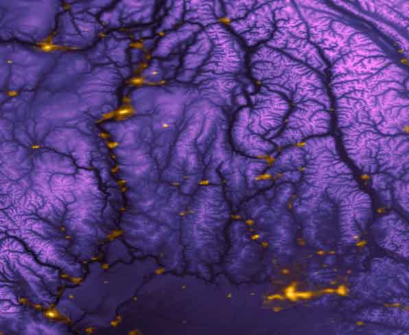
Bright cities and towns in valleys of North US and Canada.

However satellite data don’t give any direct information on the effects of this flux on the night sky due to light pollution propagation. The aim of our work is to study these effects. 

Satellite data reduction

The DMSP satellite F12 is in a low earth polar orbit and carries an oscillating scan radiometer, the Operational Linescan System, with a photomultiplier tube (PMT) as detector. The OLS scans a narrow swath of the Earth, about 3,000 km wide, perpendicular to the orbit and as the satellite moves it constructs a bi-dimensional image of the Earth surface.

What we basically do is a composition of data obtained with different gains in order to improve dynamic range and to avoid saturation. Our data have a pixel size of 30”x30” (less than 1 km) in a latitude/longitude projection. The reduction steps include: (i) detection of cloud-free areas on infrared data; (ii) cleaning; (iii) calibration based on pre-fly radiance calibration of the OLS-PMT (we checked it comparing map prediction with observations and obtained a good agreement); (iv) Richardson–Lucy deconvolution to improve prediction for sites near the sources. We pass from the radiance measured from the satellite to the intensity emission in V band from each land area covered by a pixel, accounting for atmospheric extinction, the average spectrum of night time lighting and the surface of the area. However we need not only the intensity toward the satellite but also the intensity in every other direction. We obtain the average upward emission function by studying the emission per inhabitant of many sources at different distances from the satellite nadir, seen by the satellite under different angles. We can obtain this function for each land area corresponding to each pixel, using a large number of individual orbit data. This kind of study can be done only with a non geo-stationary satellite like DMSP satellites.

Products

We obtain a number of different products which can be used for many purposes. Here a short description:

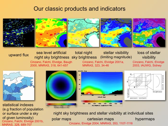
1) Maps of the upward light flux.

They are the simplest kind of map and show the total light flux emitted upward by the sources on the Earth surface and introducted  in the atmosphere.

Map of the upward light flux from North-East Italy in 1996-1997.

They are obtained simply from the radiance calibrated data of  the DMSP satellites. The data need to be corrected for the extinction on the light in the path from the source to the satellite. When possible they are deconvolved in order to obtain a better spatial resolution. The total emitted flux must be recovered from the flux emitted toward the satellite, assuming a typical average upward emission function for all the areas or obtaining it based on measurements of each area from different elevation angles made from many individual orbits.

2) Maps of the effects of the light pollution on the night sky.

The general public frequently confuse these maps with the night-time satellite images. Satellite night-time images of the Earth show the light flux emitted upward, these maps shows the effects of this light on the night sky due to its propagation in the atmosphere and its scattering by molecules and particles.

Differences are easily recognizable e.g. in lakes, seas or desertic lands near populated areas, where there are no sources. 

.

Upward light flux (left) and its effect: the artificial night sky brightness (right).

They are black in satellite images but there is nonzero sky brightness (colour) in maps of artificial sky brightness due to light pollution propagation. Moreover  the propagation of light pollution gives them a smooth appairance even if the resolution is nearly the same. 

Upward light flux from Veneto cities measured by DMSP satellite.

Artificial night sky brightness in Veneto produced by the previous light flux.

These are the outlines of the method that we used to obtain the artificial sky brightness: (i) we divide the earth surface in land areas with the same positions  and dimensions as the projections on the earth of the pixels of the satellite image; (ii) we compute the sky brightness seen in the chosen sky direction at the centre of each land area adding the contributions produced by all the areas inside a radius of 200km (for darkest sites we use 300km). The contributions are computed using the Garstang Modelling Technique (Garstang 1986, 1889a,b, 1991,1999, etc.; Cinzano 1999a,b,c) in few steps: a) We compute the light emitted by the source area and arriving to an infinitesimal volume of atmosphere along the line of sight of an observer, accounting for the extinction in the path; b) we account for light arriving in the volume after a previous scattering, for the earth curvature which shields part of the line of sight and, in some maps, for the screening due to terrain elevation and mountains; c) we compute the light scattered by molecules and aerosols in the volume towards the observer and the quantity of light arriving to the observer, accounting for extinction in this path too; d) we integrate along the line of sight. 

The resolution of the maps, depending on the results of an integration over a large zone, is greater than the resolution of the original images and is generally of the order of the distance between two pixel centres (30''x30'', i.e. < 1 km).  

The beautiful city of Venice send upward a very limited amount of light in comparison with other cities of the same population, due at its "romantic" lighting park (left image: Venice at low right and Mestre at upper left). Venice's zenith sky is imbedded in the pollution produced by Mestre and other cities (right image) but, however, it is still not much bright. Let's save the romantic low-intensity lighting of Venice!

a) Maps of the sea level artificial night sky brightness

The maps of the artificial night sky brightness at zenith at sea level allow to compare levels of light pollution in the atmosphere, to recognize more and less polluted areas and to identify the more polluting districts and the bigger sources.

These maps are intended to show the levels of pollution in the atmosphere rather than the stellar visibility which is the aim of the other maps described afterwards. The assumption of sea level and standard clear atmospherical conditions allows to compare pollution of different areas, to recognize more polluting sources or darker areas (areas with less light in the atmosphere and not areas where you see better the stars) without be confused by the altitude effects. 

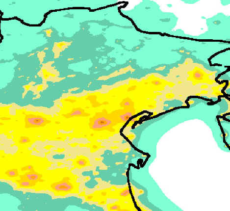
Map of the artificial night sky brightness in North-East Italy.

However you do not see a big difference accounting for altitude (e.g. in correspondence of Mount Ekar, at the borders of the padana plane, rising from sea level to 1350 m of elevation the artificial sky brightness diminishes less than about 20% whereas color levels in our maps shows each one three times larger brightness than the previous one.)

These maps do not give information on the star visibility, however mainly polluted areas usually are at sea level, so very approximately we can say that the orange level in our standard scale indicates areas where the milky way is not visible anymore. The red areas very approximately indicates zones where less than 100 stars are visible over 30 degrees of elevation. Blue border indicates artificial sky brightness over 10% than the natural brightness which is the definition of "light polluted sky". Yellow indicates an artificial sky brightness equal to the natural so that the total sky brightness is doubled.

b) Maps of the total night sky brightness

These maps of the the total night sky brightness show the quality of the night sky in the territory. They usually are computed at zenith, accounting for the elevation and the natural sky brightness. In smaller maps we also account for screening by mountain and terrain elevation. 

Map of the total night sky brightness in North-East Italy.

The elevation has effect on the natural sky brightness, on the artificial sky brightness and on the stellar extinction and is obtained from a  digital elevation map (DEM). The natural sky brightness depends on the chosen direction of view and on the altitude and it is obtained with Garstang (1989) models which account for the light coming from the entire sky and scattered along the line of sight of the observer and for the given atmospherical conditions. The mountain screening is obtained evaluating the elevation of each pixel along the line which connect each site with each source and then computing the maximum screening angle from which we determine the fraction of the line of sight shielded. This is very time consuming, in particular if the line of sight is not vertical and requires computation for each of its points.  

c) Maps of the star visibility (naked eye limiting magnitude)

The maps of the stellar visibility (naked eye limiting magnitude) show the capability of the population to see the stars. They usually are computed at zenith, accounting for the extinction of the star light in the atmosphere from the top of the atmosphere to the observer and the eye capability to detect point sources over a light background. They are unsuitable to evaluate the light pollution of the atmosphere because the elevation and extinction of the light confuse the behaviour.

As an example, the mountains near the top of the image below could appear unpolluted because they have the same limiting magnitude than unpolluted zones of the sea at lover left corner. However the stellar extinction from an elevated site is less than from sea level and the number of particles and molecules which can scatter the artificial light is less too, so that limiting magnitude and stellar visibility increase with elevation. In conclusion the similar limiting magnitude in the mountains and in the unpolluted areas of the sea implies that the mountains are polluted SO MUCH that the stellar visibility there is comparable with the visibility from sea level. In fact the subsequent figure, a map of the "magnitude loss", shows the large differences between the mountains and the sea.

Map of the naked eye limiting magnitude in North-East Italy.

As Blackwell (1946) and many other authors showed, the relation between limiting magnitude and sky brightness is not linear and, moreover, it is a statistical concept. A number of random factors affect eye measurements (Garstang 2000; Schaefer 1991) like the individual eye capability, the individual pupil size, the experience that makes the observer confident of a detection at a probability level different from another, the duration of the observation and so on. So we can predict only the star visibility by an average observer even if we account for many details (e.g. observer pupil diameter depending on the age; Stiles-Crawford effect (a decrease of the efficiency in detecting photons with the distance from the centre of the pupil); colour differences between the laboratory sources and the observed star; colour differences between the laboratory sources and the night sky; differences between the night vision curve and the V band in computing the stellar extinction.

d) Maps of the loss of naked eye limiting magnitude 

The maps of the loss of naked eye limiting magnitude show the loss of the capability of the population to see the stars. They are obtained simply by the difference between the map of the star visibility and a map of the same quantity evaluated assuming no light pollution in the area. The difference with the previous map is that in this case the effects of the pollutions are better shown everywhere but these maps are less useful to find the best observative sites.

Map of the loss of limiting magnitude in North-East Italy.

e) Maps of the number of visible stars

The maps of the number of visible stars shows how many stars are visible in the sky. The limiting magnitude can be related to the number of star which are visible in the sky but a detailed computation requires an evaluation of the stellar visibility in each direction of the sky and not only at the zenith, accounting for the increase of the stellar extinction with the zenith distance. This requires an incredible amount of computational time. This kind of maps are still under study.

f) Maps of the loss of visible stars 

The maps of the loss of visible stars are simply obtained by difference between the map of the number of visible stars and a map of the same quantity evaluated assuming no light pollution in the area. Like the maps of the loss of naked eye limiting magnitude, these maps shows better the effects of the light pollution but are less useful to evaluate the capability of the population to see the stars.

3) predictions of the future effects of the light pollution on the night sky.

We are studying the effects of the increase of light pollution which is exponential almost everywhere with average yearly growth rates as large as 5%-10% measured both in US and Europe. Some projections have been already made for Europe and North America.

Growth of the night sky brightness in Veneto 1971-2025

4) Maps of tHE ENTIRE SKY OF INDIVIDUAL SITES.

The maps of the entire sky of individual sites can be obtained with an analogous method. We make maps of the artificial night sky brightness, the total night sky brightness and the naked eye limiting magnitude. All of them account for elevation, mountain and terrain screening, Earth curvature, atmospheric conditions, etc.